Wednesday Football Post: Revisiting Pythagorean Wins

Delving into the method behind the madness of Pythagorean Wins

Editors Note: I am aware that I said the first return post would be on 2/1. That was a lie, because I realized I could do this and wanted to talk about it. Enjoy the extra content.

Pythagorean Win Percentage (PWP), using a team’s points scored and points allowed to predict their win percentage, was first presented for Major League baseball sabermetrician Bill James in his 1980 edition of Baseball Abstract. This elegant idea has since been replicated in the other major American sports, notably by Daryl Morey, with particular attention given to what exponential constant to use to best predict win percentage. While I do arrive at several estimates for the NFL (2.77), Power 5 FBS (2.21), Group of 5 FBS (2.31), NBA (14.2), and NHL (2.10), and I want to focus on how to arrive at these estimates.

The general form of PWP is as follows:

The Pythagorean part of the name came about not because it is derived from triangles — although it has been derived it from first principles — but because James set k = 2 in the first iteration making it look like A^2 + B^2 = C^2. While it would make sense in some contexts to consider Points Allowed to be negative, we consider it to be a positive here.

This formula will always yield a number between 0 and 1. The best a team can do is score points while allowing no points, yielding 100%. The worst a team can do is score 0 points while allowing points, yielding 0%. As long as k > 0, this key behavior will remain intact. What changes with k, however is that larger k values cause the to approach 100% or 0% with the same points scored and allowed quicker.

For a concrete example, take the 2022 New England Patriots. Overall they were a solid squad with an inconsistent offense and managed to stay in the playoff hunt until the last week of the season. They ended up finishing just below 0.500 at 8-9. To illustrate the difference a k value can make, we’ll use their 364 points scored and 347 points allowed to see what expected win probability will pop out at two extreme k values: 1 and 15.

With k = 1, we get an estimate which says the Patriots should’ve won a little more based on their scoring than they lost and implies they won about 0.7 less games than they should have. This feels like a reasonable estimate overall. When we crank k all the way up to 15, however, our result suggest the Patriots got jobbed out of nearly 3.5 wins. This is probably an overly optimistic expectation and we need a better estimate. Our k should probably be somewhere in the middle, but how do we figure it out?

The most straight-forward way would be to test a bunch of different k values within a reasonable range, plug them in, and find which one gives us the smallest error. This could certainly work, and we could even devise clever ways to pick k values to save computing time to counteract the obvious drawbacks of this approach. This is a valid approach ,and would likely yield a good estimate for k, but it wouldn’t meaningfully leverage the empirical data we have at hand nor take advantage of our available definition. We can circumvent both of these problems by doing some algebra on our original equation to isolate k. We end up with the following:

This is very gross looking and annoying to workout if you don’t use Wolfram Alpha, but the important part is that everything inside of the disgusting logarithms is constant. That means with every observation we have (a team in a season) we can calculate it right away and are left with something that looks like b = ak, a classic linear regression! If we regress our new terms, which are calculated from data we already have, against each other, then the slope we get is an empirical estimate for k.

I am not the first to use this method. It has been the standard for nearly 20 years according to John Chen and Tengfei Li in The Shrinkage of the Pythagorean exponents. I just hope to explain it to you in more ordinary language and share further details of results.

Great! So we have an empirical estimate from a regression with the added benefit of a margin of error as a result, which makes it more flexible than a plug-and-chugged estimate. But does this k estimate actually outperform just testing a bunch of values?

Looking at the three major error measures (Root Mean Square Error, Mean Absolute Error, and Mean Squared Error), our regression estimate for the NFL is slightly higher than those yielded by plugging and chugging according to RMSE, MAE, and MSE. But all of the plug and chug results are within our margin of error from our regression results, giving us strong reason to trust our regression result. Since this is a regression, it is sensitive to the time period we choose. For the purposes of this exercise I chose 2002-2022 as that is the period of time in which the NFL has had 32 teams, but this is arbitrary. For more actionable purposes it may be more reasonable to choose 5-10 year windows to better reflect the league in its current state, whenever that may be.

Does a similar analysis hold for the other leagues mentioned earlier?

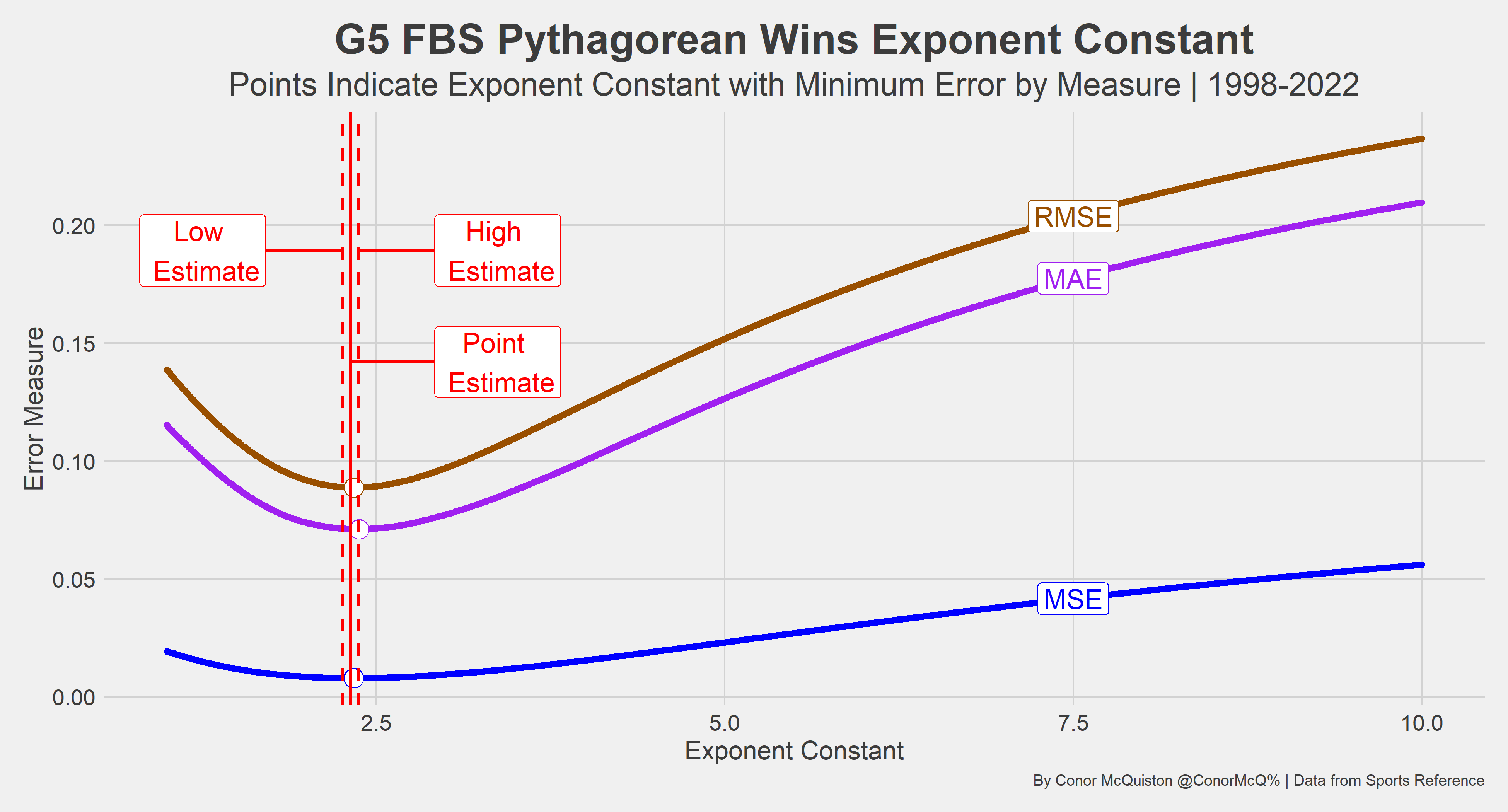
It does overall! The weakest are certainly the CFB estimates, which is understandable since my decision to split G5 and P5 FBS football was based on nothing more than my intuition that G5 points allowed may be inflated from occasional shellackings from P5 foes. Even with this easily to argue down consideration, the regression still performed well and is one of the easiest ways to determine the optimal k value in Pythagorean Win Probability constructions.

Thank you for reading and I hope you enjoyed! Talk to you next week when we’ll connect recruiting stars to the Pro Bowl and All-Pro Teams! -CRM